Visualizing geographic data with folium, the bike ride case part 2
- jercoli

- Feb 15, 2021
- 4 min read
Hello, we continue to analyze our data on bicycle trips of the public service in the city of Buenos Aires, Argentina. In this case we will concentrate on a data visualization project, more precisely on the representation of certain data on a geographic map. For this we will use a powerful library of geographic representation: Folium
Folium "builds on the data wrangling strengths of the Python ecosystem and the mapping strengths of the leaflet.js library" Folium creates a map in a separate HTML file, but in case you use Jupyter notebook (like myself), you might prefer to get inline maps.
The objective will be to visualize the origin and destination stations on the map, represented by a circle and the journey route represented by a line. Also above the line the amount of trips made between the two stations should be displayed.
First we import the necessary libraries and access our data in google drive ( it is advisable to read the first part in this post )
import matplotlib.pyplot as plt
import pandas as pd
import numpy as np
import folium
%matplotlib notebook
from google.colab import drive
drive.mount('/gdrive')
%cd /gdrive/My Drive
# create the dataframe from csv data
bike_ride_2018 = pd.read_csv('./BA-bikes-rides-2018.csv')
Reformat some data, change NaN values (an acronym for Not a Number) and create a new index
# put -1 in NaN values
bike_ride_2018 = bike_ride_2018.fillna(-1)
# rename and convert to int some columns
bike_ride_2018.rename(columns={'fecha_origen_recorrido':'dateTime'}, inplace=True)
bike_ride_2018['id_estacion_origen'] = bike_ride_2018['id_estacion_origen'].astype(int)
bike_ride_2018['id_estacion_destino'] = bike_ride_2018['id_estacion_destino'].astype(int)
# create new index type date
bike_ride_2018['date'] = pd.to_datetime(bike_ride_2018['dateTime']).dt.date
bike_ride_2018.set_index('date', inplace=True)
bike_ride_2018.head()
Now we will create a new dataframe with partial data from the original bike_ride_2018 df, in this way we will be able to speed up the processing times and test our procedures in a more agile way.
It is very common in jupyter notebooks to create new dataframes from others, and in this way keep the original ones in case we have to start new data analysis branches from there.
# create new df for only a month of bike_ride_2018, to process my tests faster
start_date = '2018-01-01'
end_date = '2018-01-31'
mask  =  ( bike_ride_2018[ 'dateTime' ]  >= start_date )  &  ( bike_ride_2018[ 'dateTime' ]  <=  end_date )
br_2018_net = bike_ride_2018.loc[mask]
#reset the index to default (int)
br_2018_net.reset_index(drop=True, inplace=True)
#print(f"Rows: {br_2018_net.size}")
br_2018_net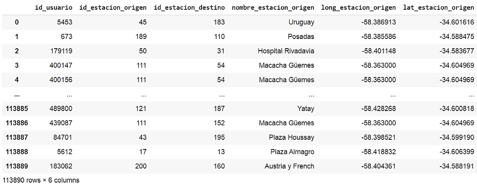
Ok we have 113890 rows, now we will delete from our dataframe those rows that contain stations with id equal to -1
# Drop all the stations that have -1 in your id
br_2018_net = br_2018_net.drop(br_2018_net[(br_2018_net['id_estacion_origen'] == -1) | (br_2018_net['id_estacion_destino'] == -1)].index)
br_2018_net
And then 110744 rows remain
So far we have our clean data from which we must obtain :
the stations (unique, without repeating)
the trips between them
For this we will create 3 new dataframes, one with the origin stations, another with the destination stations and the last with the number of trips between them. Finally we will unite them in a single dataframe
# create new df only with origin bike stations
origin_stations = br_2018_net[['id_estacion_origen','nombre_estacion_origen','long_estacion_origen', 'lat_estacion_origen']].drop_duplicates().reset_index()
origin_stations.rename(columns={'id_estacion_origen':'station_id_o', 'nombre_estacion_origen':'station_o', 'long_estacion_origen':'long_o', 'lat_estacion_origen':'lat_o'}, inplace=True)
origin_stations.drop(['index'], axis = 1, inplace=True)
origin_stations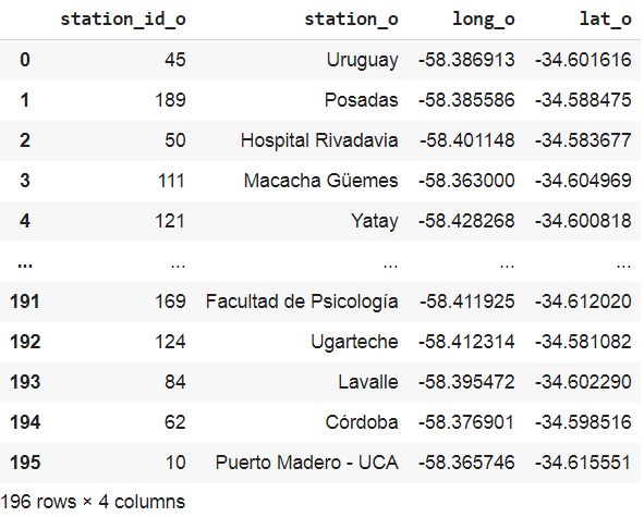
Origin stations
# create new df only with destination bike stations
destination_stations = br_2018_net[['id_estacion_destino','nombre_estacion_destino','long_estacion_destino', 'lat_estacion_destino']].drop_duplicates().reset_index()
destination_stations.rename(columns={'id_estacion_destino':'station_id_d', 'nombre_estacion_destino':'station_d', 'long_estacion_destino':'long_d', 'lat_estacion_destino':'lat_d'}, inplace=True)
destination_stations.drop(['index'], axis = 1, inplace=True)
destination_stations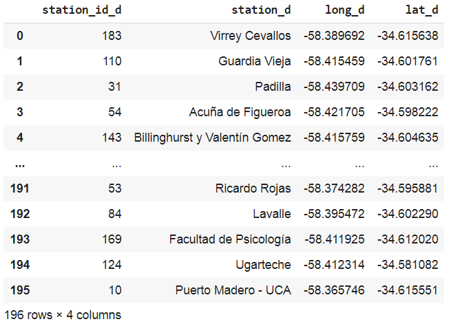
Destination stations
# calculate trips between origin and destination
count_viajes = br_2018_net.groupby(['id_estacion_origen', 'id_estacion_destino']).size()
br_2018_sum_viajes = count_viajes.to_frame(name = 'travels').reset_index()
br_2018_sum_viajes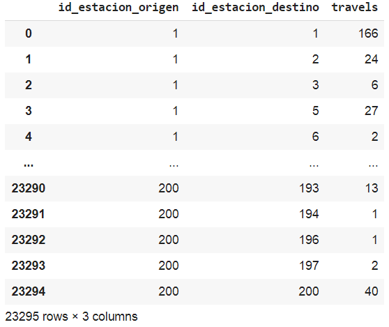
Travels between stations
# Merge with origin stations data, then with destination stations data
br_stations_travels_partial = pd.merge(left=br_2018_sum_viajes, right=origin_stations, how='left', left_on='id_estacion_origen', right_on='station_id_o')
br_stations_travels = pd.merge(left=br_stations_travels_partial, right=destination_stations, how='left', left_on='id_estacion_destino', right_on='station_id_d')
br_stations_travels
We have already gone through the hardest work !!, now we have the necessary data to be able to visualize them on the map and thus fulfill the objective of the project.
As I said before, we will use Folium to visualize the data geographically, since we have the latitude and longitude in each of the bike stations. In the code you will see that we initialize our map by centering it on the correct coordinates, select a tile (Folium have several tiles like 'openstreetmap' or 'MapQuest Open Aerial', etc) and we will also add a tool that has folium for the user to calculate distances between geographic points.
from folium import plugins
# Get a map
bike_rides_map = folium.Map(location=[-34.59, -58.39], tiles="Stamen Toner", zoom_start=15)
# Add measure tool
measure = folium.plugins.MeasureControl()
measure.add_to(bike_rides_map)
# only take the first 20 rows for display purposes
br_stations_travels = br_stations_travels.iloc[1:20]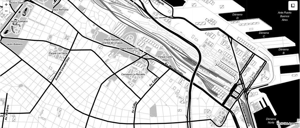
OK, now we will create the layer with the data, for visualization reasons we will only take the first 20 rows. In the code, you will see that we go through the rows to obtain:
bike stations represented by circles (folium.Circle), green for the origins and purple for the destinations (a station can have both)
lines (folium.PolyLine) connecting both travel stations
additional text (folium.PolyLineTextPath) with the number of trips to place it above the connection line.
# only take the first 20 rows for display purposes
br_stations_travels = br_stations_travels.iloc[1:20]

# iterate over df
for index, row in br_stations_travels.iterrows():

 # add origins
  folium.Circle(
    location=[row["lat_o"], row["long_o"]],
    radius=40,
    color="green",
    fill=True,
    opacity=4,
    tooltip=str(row["station_id_o"])+"-"+row["station_o"],
  ).add_to(bike_rides_map)

 # add destinations
  folium.Circle(
    location=[row["lat_d"], row["long_d"]],
    radius=50,
    tooltip=str(row["station_id_d"])+"-"+row["station_d"],
    color="#1300ca",
    fill=True,
  ).add_to(bike_rides_map)

 #add travel line origin-destination
  travel_coord = [ [row["lat_o"], row["long_o"]], [row["lat_d"], row["long_d"]] ]
  travel_line = folium.PolyLine(travel_coord, color="orange", weight=2, opacity=1,)
  travel_line.add_to(bike_rides_map)

 #add text to polyline
  attr = {'fill': 'black', 'font-weight': 'bold', 'font-size': '14'}
  text_in_line = " " * 30 + "Travels: "+str(row["travels"])+"--->"
  folium.plugins.PolyLineTextPath(travel_line, text_in_line,
                           offset=7, attributes=attr).add_to(bike_rides_map)
bike_rides_map
On the map we can position ourselves at a certain station and see its id and name. We can also activate the measurement tool and calculate the distance between 2 stations:

To download the jupyter nb: github folium example Ok folks, now is time to generate your own geographic visualization project with Folium and advance your data science career.
Your comments are appreciated


Comments